Airline Traffic Between States

Use custom made pie charts to visualize U.S. Map of State-to-State Travel

Pie charts have a rich history. William Playfair first used them in 1801, and despite decades of criticism from data visualization purists, they remain one of the most instantly recognizable ways to show proportions. Today we'll put them to work in a decidedly non-standard way: placing custom-built pie charts directly on a geographic map to reveal where Americans fly.

You can find the companion notebook on the Visualizarion for Data Science GitHub repository:

The Bureau of Transportation Statistics provides a wide range of datasets on US and global transportation infrastructure. We have used it previously here, here, and here.

The first step in our analysis is to extract the Top destinations for each state. We sort the outgoing destination of each state and extract the Top n:

Applying this function using Pandas apply gives us just the edges we need:

Matplotlib has support for pie charts, but it does not allow us to easily draw multiple pie charts in the same Axes object. To achieve this, we have to build our pie charting function from scratch by leveraging matplotlib’s Patches, 2-D shapes such as a rectangles, circles, wedges, arrows, or arbitrarily complex polygons.

We will represent each slice of the pie as a Wedge.

Our draw_pie function takes a center position, a radius, a list of fractions, and a list of colors. It loops through the fractions, converting each one into a start and end angle, then creates a Wedge patch and adds it to the current Axes:

With the function in place, we need to position the pies on a map. We'll use Cartopy for the geographic projection and map features. For each state, we look up its centroid coordinates and draw a pie chart showing the relative share of traffic to its top destinations:

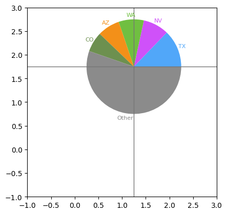
Before going all-in, it's always a good idea to test with a single state. Here's what the pie chart for one state (California) looks like on its own:

Now we can put it all together. We iterate over every state, compute the traffic fractions for its top destinations, and draw a pie chart at the corresponding location on the map. The radius of each pie is scaled by the total traffic volume, so busier states get larger charts:

And here's the result — a full map of the continental U.S. with pie charts showing the top 5 destinations from each state:

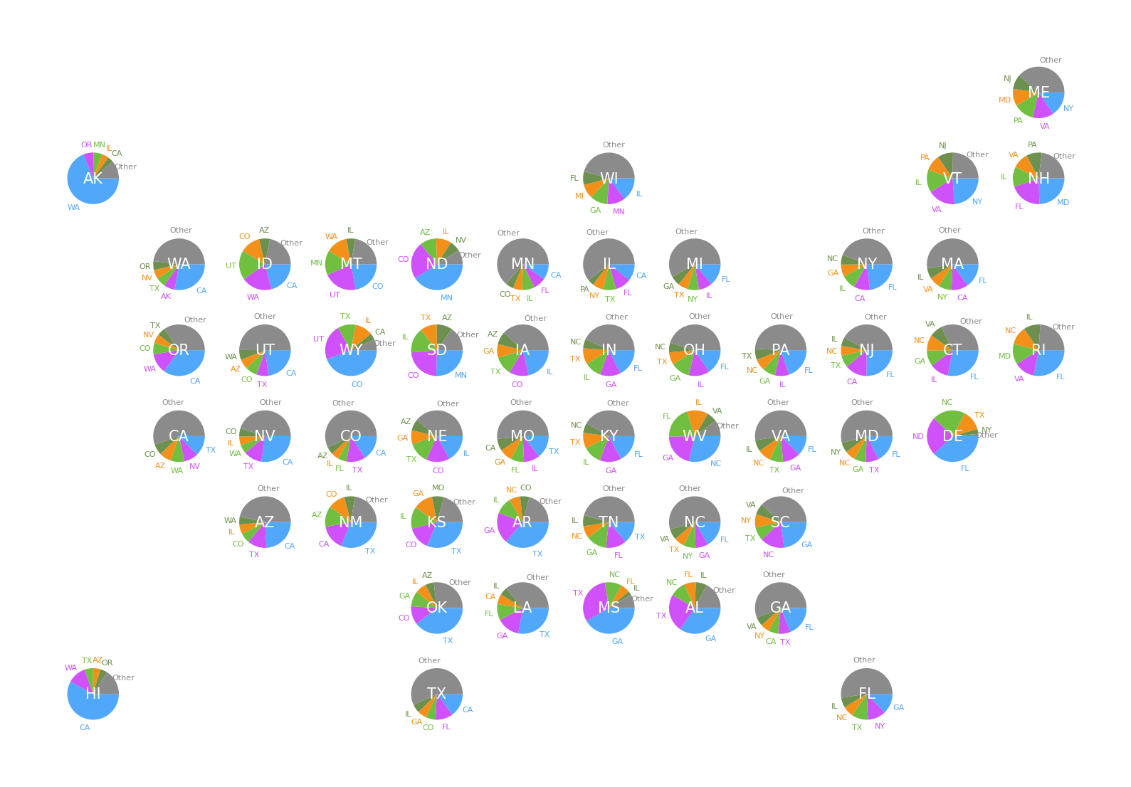
The visualization is already revealing. States like California and Texas have large, diverse pie charts, while smaller states show more concentrated travel patterns — often dominated by a single hub. But what happens when we increase the number of destinations? Let's bump it up to the top 10 and see how the picture changes:

With more slices in each pie, the regional patterns become even clearer. Neighboring states often share the same dominant destinations, creating natural clusters of travel corridors:

What stands out most is how geography shapes air travel. Coastal states connect to distant hubs — New York, Los Angeles, Chicago — while states in the middle of the country funnel traffic through regional powerhouses like Dallas and Denver. The pie charts make these patterns immediately visible in a way that a simple table of numbers never could.

We hope you enjoyed this Visualization post on the Data for Science Substack and look forward to hearing your thoughts. We hope you

You can find all the code for the analysis in this post in our companion GitHub Repository

And, of course, don’t forget to

this post with others who might be interested, and encourage them to

so that they have access to the entire backlog of posts and be the first to know when a new a new article is posted.