

Build a (small) language model by counting
A 4-gram model on WikiText-103, and the one idea it shares with Claude.

This week we continue our exploration of Large Language Models by building a simple markov based language model. By the end of this post you’ll understand better the basic mechanisms underlying language generation.
You can also find the companion notebook on the LLMs for Data Science GitHub repository:
You can also find the companion notebook on the LLMs for Data Science GitHub repository:

Every language model does one thing. It reads some words and guesses the next one. ChatGPT does it. Your phone keyboard does it. The model in this post does it too, and you can build this one by hand. It counts how often each three-word sequence is followed by a given word, then turns those counts into probabilities. That single idea, next-word prediction, sits at the center of every system in the field.
The build is short. We start with what an n-gram model is and where the idea came from. We load WikiText-103 and study it. We build the model, read off what it learned, and let it write. We close by setting this counting model next to a neural network and naming what changes at scale.
What a language model does
A language model answers one question. Given some words, what word comes next? Feed it “the United States of” and a good model puts high probability on “America”. Feed it “I poured milk into my” and it favors “coffee” or “cereal” over “elephant”. The model holds no facts in any deep sense. It holds how often words follow other words.
Write this as a probability. For a run of words w1 to wT, the model gives the chance of the whole run:
Each factor is the chance of one word given everything before it. The product rule turns a sentence into a chain of next-word guesses. That chain is the whole job. The rest is detail about how we get those probabilities.
The Markov shortcut
The full history is too long to count. The phrase “everything before it” can run to thousands of words, and most long phrases show up once or never. Andrey Markov hit this wall in 1913. He studied letter patterns in Pushkin’s Eugene Onegin and made a bold cut. He assumed the next item follows from a short window of recent items, not the entire past.
An n-gram model takes that cut. It keeps the last n-1 words and drops the rest:
A unigram keeps no context and counts raw word frequency. A bigram keeps one previous word. A trigram keeps two. The model here keeps three previous words and predicts the fourth, so it is a 4-gram model.
Counting gives the probabilities
How do we get the numbers? We count. To estimate the chance that “States” follows “the United”, divide two counts:
That ratio is the maximum likelihood estimate. The best guess for the next word is what we saw, weighted by frequency. Tally these counts over a large body of text and you have an n-gram model. No training loop. No gradient descent. Just tallies.
A long track record
The idea is old and it worked. Claude Shannon used n-gram models of English in his 1948 paper that founded information theory. He showed that letter and word n-grams could mimic the texture of real writing. By the late 1980s, teams at IBM ran n-gram models with millions of counts for speech recognition and machine translation. In 2006 Google released a 5-gram dataset drawn from a trillion words of web text. For decades the n-gram was the workhorse of language technology.
Where n-grams break
Two problems limit the n-gram, and the data study below shows both. The first is sparsity. Language has a long tail. Most word combinations are rare, and most possible n-grams never appear in any corpus. A 4-gram model trained on a hundred million words still meets fresh four-word runs at test time and hands them probability zero.
The second problem is blindness to meaning. The n-gram treats “dog” and “puppy” as unrelated symbols. It learns nothing about “the happy puppy ran” from having seen “the happy dog ran”. Each count stands alone. A model that cannot share what it knows across similar words needs to see every phrasing on its own, and no corpus is that big.
These two cracks are the reason neural language models exist. We come back to that after the build.
The data: WikiText-103
We build on WikiText-103, a standard benchmark drawn from Wikipedia articles that editors marked Good or Featured. The training split holds about 103 million words across roughly 28,000 articles. We use the raw build, which keeps the original capitalization and punctuation and hides nothing behind a placeholder token.
wikitext = load_dataset(”wikitext”, “wikitext-103-raw-v1”, split=”train”)The split arrives as 1,801,350 rows. Each row is one line of an article, a heading, or a blank separator. About 35 percent of the rows are blank, which leaves 1,165,029 rows of real text.
How long are the rows?
Word counts per row show how the text is chunked. Headings are short. Paragraphs run long. Tokenizing all 1.8 million rows takes minutes, so the data study draws a sample of 20,000 non-blank rows. That sample holds 1,758,094 tokens. The mean row runs 87.9 tokens, the median 75, and the longest row in the sample reaches 711.
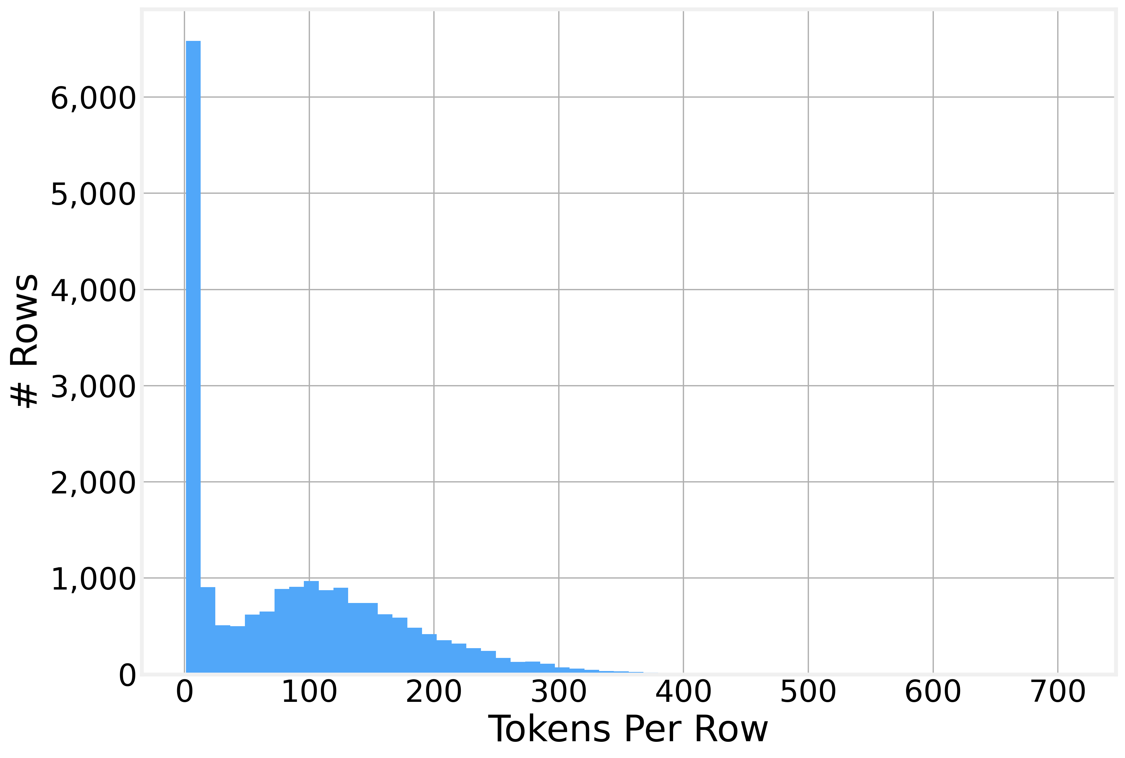
The histogram leans hard to the left. Most rows are short. A thin tail stretches out to the long paragraphs.
Which words appear most?
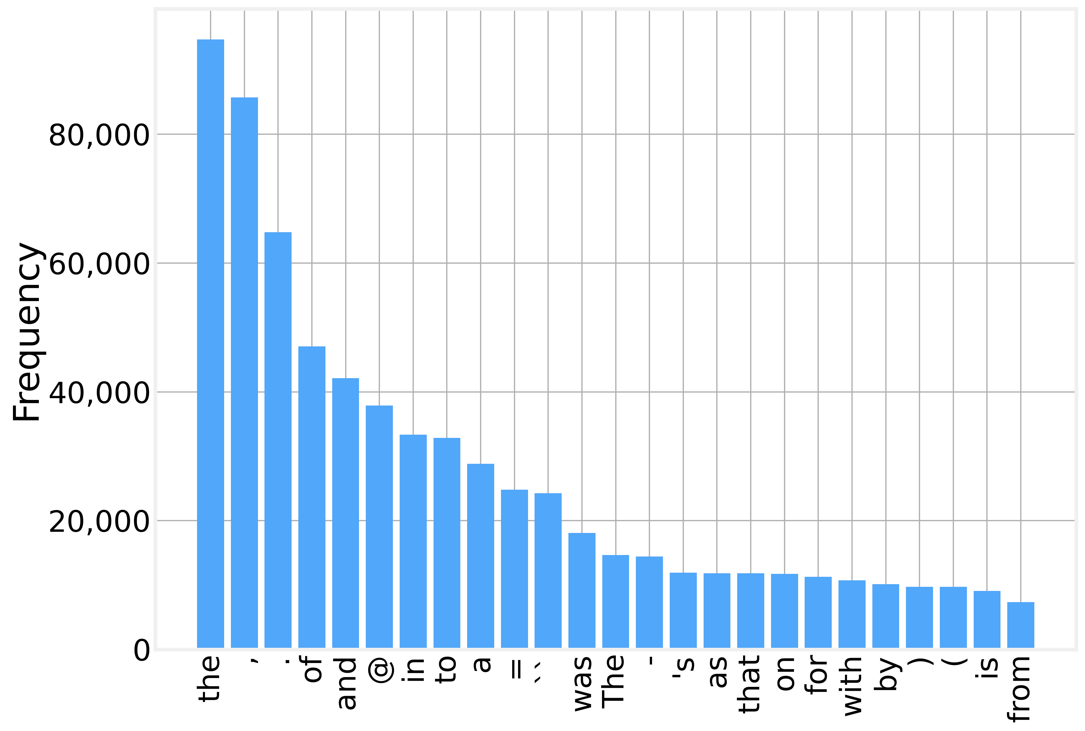
Pool the sampled tokens into one counter and the top of the list holds no surprise. Function words and punctuation lead. The word “the” comes first, then the comma, the period, “of”, and “and”. The sample holds 68,641 distinct word types across those 1.76 million tokens. The bottom of the list is a long tail of names, numbers, and rare terms that each show up once.
Zipf’s law
Word frequencies fall in a steep, regular pattern. Rank the words from most to least common, then plot rank against frequency on log-log axes. The points sit along a near-straight line. The most common word lands about twice as often as the second, three times as often as the third, on down the list. This is Zipf’s law, and it holds across languages and corpora.
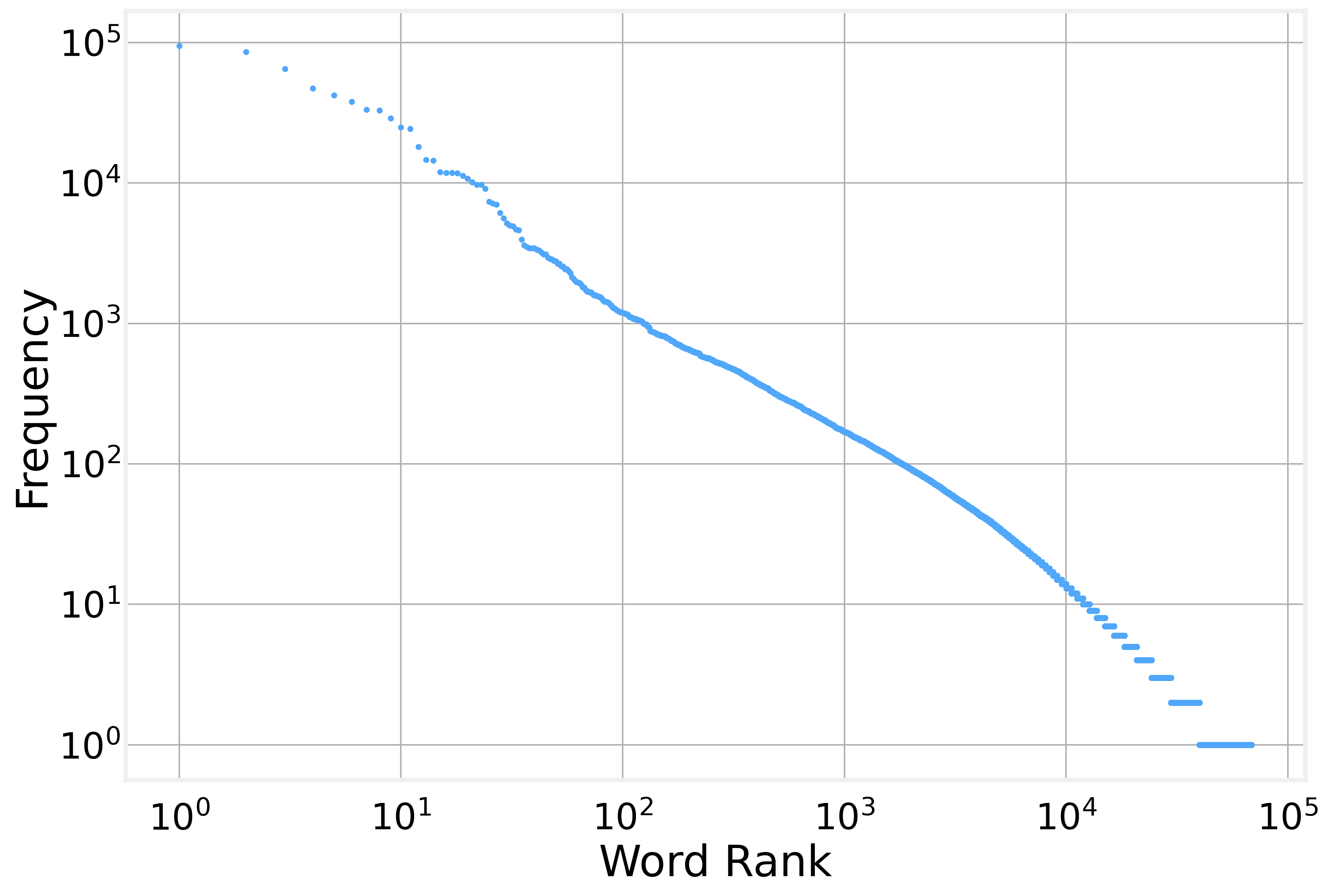
Zipf’s law is the root of the sparsity problem. A few words cover most of the text. The rest are rare. Any model that counts word combinations will meet most combinations too few times to trust.
Counting the contexts
The model rests on three-word contexts, so count those directly. In the sampled text, how many distinct three-word contexts appear, and how many words follow each one? The sample holds 1,243,344 distinct contexts. Of those, 1,121,597 carry exactly one continuation. That is 90.2 percent. The mean context offers 1.25 next words. One context, a very common one, offers 3,875.
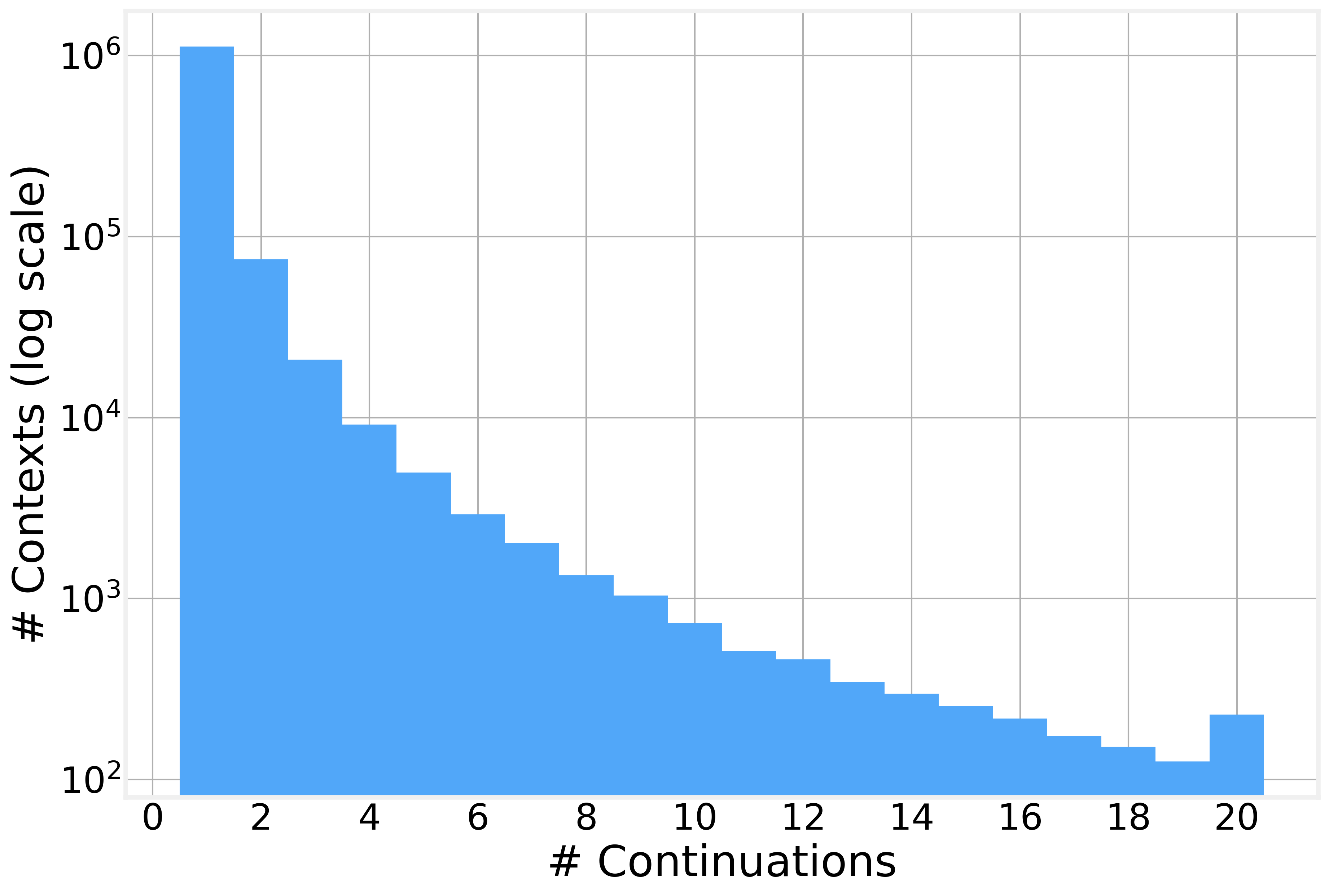
Read that number again. Nine in ten contexts saw a single word follow, so the model has no real choice for them. It repeats what it saw. Only the common contexts give several options with spread-out weight. This split is the reason the generator sounds fluent in short bursts and slides into copied text over longer runs.
Building the model
Now we build the full 4-gram model over the whole training split, not the sample. At each position we record the three-word context and the word that follows. NLTK pads the ends so the first and last words get full contexts. The full pass over 103 million words runs for a few minutes, and we cache the finished table to disk.
model = defaultdict(next_word_counts)

for item in tqdm(wikitext, desc="Counting 4-grams"):
    text = item["text"]
    if not text.strip():
        continue
    tokens = word_tokenize(text)
    for w1, w2, w3, w4 in ngrams(tokens, 4, pad_right=True, pad_left=True):
        context = (w1, w2, w3)
        model[context][w4] += 1
The finished table holds 41,277,266 distinct contexts. That is the full memory of the model, every three-word window the corpus ever showed.
We turn the raw counts into probabilities. For each context, divide every next-word count by the total for that context. The numbers for each context now sum to one.
for context in model:
    total_count = float(sum(model[context].values()))
    for word in model[context]:
        model[context][word] /= total_count
Read off the context “the United States” and you see the model’s guess for the fourth word.
model[(”the”, “United”, “States”)]A period comes next 18 percent of the time. A comma 17.5 percent. The word “and” 7 percent, “on” 7 percent, “Army” 2 percent, “Navy” 2 percent. The distribution mixes punctuation, function words, and a crowd of proper nouns tied to the phrase. That spread is the model in one glance.
Generating text
Now we let the model write. Start from a three-word prompt and ask for the next word. Append it, slide the context forward by one, and ask again. Repeat until the model emits the end marker. This loop, feed the output back in and predict the next token, is autoregressive generation. It is the same loop that runs inside every large language model.
The function has a temperature switch. With temperature off, it always takes the single most likely next word. That is greedy decoding. With temperature on, it samples a word in proportion to the probabilities, so rare words get an occasional turn. Large models expose the same knob. Low temperature gives safe, repeating text. Higher temperature gives variety and surprise.
def generate_sentence_from_prompt(model, prompt, zero_temperature=False):
    text = [*prompt]

    while True:
        # The current context is the last three words of the running text.
        context = tuple(text[-3:])

        # An unseen context has no continuations. Stop if we land on one.
        if context not in model:
            break

        # Pull the candidate next words and their probabilities.
        words = []
        probs = []
        for word, prob in model[context].items():
            words.append(word)
            probs.append(prob)

        if zero_temperature:
            # Always take the most likely word. Temperature = 0.
            pos = np.argmax(probs)
        else:
            # Sample one word in proportion to its probability. Temperature = 1.
            selection = np.random.multinomial(1, probs)
            pos = np.argmax(selection)

        word = words[pos]
        text.append(word)

        # Three None tokens in a row mark the end of a sentence. Stop there.
        if text[-3:] == [None, None, None]:
            break

        # Guard against a runaway greedy loop.
        if zero_temperature and len(text) > 100:
            break

    return " ".join([t for t in text if t])
Start from “United Kingdom of” and sample, and the model stitches real fragments into a line that reads well for a clause and then drifts:
United Kingdom of Great Britain at the 1948 Democratic National Convention
in Denver , Co . Rd . AAA . The grant was contingent upon German economic recovery .
The same prompt at two temperatures makes the contrast plain:
prompt = ("the", "United", "States")

print("Greedy (temperature = 0):")
print(generate_sentence_from_prompt(model, prompt, zero_temperature=True))

print("\nSampled (temperature = 1):")
print(generate_sentence_from_prompt(model, prompt))
Greedy decoding walks the single most common path and collapses almost at once:
the United States .
Sampling stays varied and wanders through the corpus:
the United States , designed to handle , and as of 23 April 1918 = = = Severe Tropical Storm Fern was a damaging race , and to a lesser extent , Alaska cedar . Devil ‘s Punch Bowl , located south of Baja California Sur . The hurricane dropped additional heavy rainfall ...
The text reads fluently for a clause, then jumps topic at every context boundary. The “= = =” marks are a section heading the model copied whole. The “@-@” tokens you will see in other runs are WikiText’s encoding for hyphenated words, left in raw.
From this model to Claude
The model in this post and a system like GPT-4 solve the same task. Both read some tokens and predict the next one. Both write by the same loop, one token at a time, feeding each output back as input. Both pick from a probability distribution and use a temperature setting to trade safety for variety. The job is identical. What changed is how the probabilities get computed.
Three differences carry most of the weight.
Context length. Our model looks at three words and forgets the rest. A modern transformer reads thousands of tokens at once and can attend to any of them. It can tie a pronoun back to a name twenty sentences earlier. The n-gram cannot see past its tiny window.
Representation. Our model stores raw counts in a lookup table. The words “dog” and “puppy” are separate keys with nothing in common. A neural model maps each word to a vector of numbers learned from data. Words used in similar ways land near each other in that space. A neural model can score “the happy puppy ran” from patterns it picked up on “the happy dog ran”. The n-gram learns each phrasing on its own.
Generalization to the unseen. Our model hands probability zero to any context it never saw, which breaks generation the moment it meets something new. A neural model spreads probability across all words and never returns a hard zero. It guesses sensibly on input it has never met.
Scale ties these together. This model holds a table built from 103 million words. Current state of the art models hold on the order of trillions of learned weights and are trained on tens of trillions of tokens. The jump from counting to neural networks did not change the question. It changed the answer from a static tally into a learned function that shares knowledge across words and reaches across long context.
Despite recent developments, the n-gram is not dead history. Its assumptions are plain, it builds in a single pass with no special hardware, and it still serves well for spelling correction, simple autocomplete, and as a fast baseline. The point of this walk is the line that runs from it to the largest models. Predict the next token, sample, repeat. Every advance after that point is a richer way to compute that one probability.
We hope you enjoyed the very first LLMs post on the Data for Science Substack and look forward to hearing your thoughts. We hope you
You can find all the code for the analysis in this post in our brand new companion GitHub Repository https://github.com/DataForScience/LLMs
And, of course, don’t forget to
this post with others who might be interested, and encourage them to
so that they have access to the entire backlog of posts and be the first to know when a new a new article is posted.