


Welcome to the latest post in the Graphs for Data Science substack. In this post, we explore the fundamentals of Graph Neural Networks using a fascinating dataset on molecular structures.
As always, you can find the companion notebook on the Graphs for Data Science GitHub repository:

In this post, we’re flipping our usual script, and instead of focusing on analyzing a graph, we’re going to learn from one. We’ll build a neural network to predict a molecule's solubility in water purely from the graph structure of the connections between atoms. The family of models that pulls this off goes by the name Graph Neural Networks (GNNs), and they’ve quietly become one of the most versatile tools in the modern ML toolkit.
For the sake of convenience (and a shiny new dataset), we’re using molecules as our playground. Still, the core ideas: message passing, neighborhood aggregation, and graph-level readout are applicable anywhere you encounter graph structure: social networks, road systems, knowledge graphs, protein interactions, you name it.
Why Graph Neural Networks?
If you’re a data scientist, you already have great intuitions for images and text. Images are a grid of pixels, and CNNs exploit that grid by sliding small filters across it. Text is a sequence of tokens that Transformers and RNNs can leverage.
Now look back to your high school chemistry class and think about everyones favorite molecule, Caffeine: 14 heavy atoms in a fused ring system.

There’s no natural “first pixel” or “first token” here. The atoms have no inherent order. The connectivity pattern is a graph.
You *could* try to flatten a molecule into a fixed-length vector. That’s exactly what traditional molecular fingerprints do: walk the graph, hash substructures, and pack everything into a bit vector. It works okay, but you’re throwing away structural information in the process. Atoms that are three hops apart in the molecular graph end up jumbled with their direct neighbors. The representation has no idea who’s bonded to whom.
GNNs take a different approach. They operate directly on the graph, respecting its topology. Every atom “talks” (sends messages) to its neighbors, and the network learns which conversations matter and which ones don’t.
Naturally, these same ideas are applicable well beyond molecules. Traditional Neural networks struggle with *any* graph-structured data for three fundamental reasons:
Variable size: different graphs have different numbers of nodes and edges. You can’t just reshape them into a nicely shaped tensor
No natural ordering: unlike pixels in a grid or words in a sentence, graph nodes have no inherent sequence.
Complex relationships: information flows along edges in patterns that don’t map neatly onto convolutions or recurrence.
GNNs were designed from the ground up to handle all three of these challenges.
Message Passing: A Game of Telephone
The main idea at the heart of every GNN couldn’t be simpler, just message passing (typically known to physicists as Believe Propagation). Think of it like a game of telephone, where you’re an atom sitting inside a molecule. You start with an initial feature vector that describes you: your element type, how many bonds you have, whether you’re part of an aromatic ring, your formal charge, and so on.
Now, at each step, you:
Collect the feature vectors (messages) of all your neighbors
Aggregate those messages by summing, averaging, etc.
Update your own representation by combining what you just learned with what you already knew
After one round, you know about your immediate neighborhood. After two rounds, you know about your neighbors’ neighbors. After k rounds, your representation encodes information from your entire k-hop neighborhood. It’s like each atom gradually building up a richer and richer picture of its local chemical environment.
Mathematically, this looks like:
where h_v^l is the feature vector of node v in layer l, and N(v) is the set of its neighbors. The AGGREGATE function collects information from the neighborhood, and UPDATE combines it with the node’s current state.
The GCN Flavor
The specific architecture we’ll build today is the Graph Convolutional Network (GCN), introduced by Kipf and Welling in their influential 2017 paper. The GCN makes a particularly clean choice: aggregate by taking a normalized sum of linearly transformed neighbor features.
Each neighbor’s features get multiplied by a learnable weight matrix W, then we sum up all those transformed vectors, while scaling each one by
where k is the node degree to prevent high-degree nodes from dominating the aggregation. This is essentially the graph equivalent of batch normalization: a small detail that makes training dramatically more stable.
Finally, f is any nonlinear activation function (we’ll use ReLU), which lets the model learn non-trivial relationships between features.
Alternative GNN Architectures
While we’re building a GCN today, it’s worth knowing that there are many other versions out there:
Graph Attention Networks (GATs): Learn attention weights so the model can determine which neighbors matter most for each node. More expressive, but computationally heavier.
GraphSAGE: Samples from a fixed number of neighbors instead of using all of them, making it possible to scale to millions or billions of nodes.
Graph Isomorphism Network (GIN): Maximizes expressiveness within the message-passing framework, matching the power of the Weisfeiler-Leman graph isomorphism test.
Message Passing Neural Networks (MPNN): Explicitly separates the message, aggregation, and update steps, encompassing most other architectures as special cases.
But they all correspond to different ways of choosing those AGGREGATE and UPDATE functions.
Our Dataset: Predicting How Well Molecules Dissolve
We’ll use the ESOL (Estimated SOLubility) dataset from the MoleculeNet benchmark. The ESOL contains information on 1,128 small organic molecules, each labeled with how well the molecule dissolves in water, expressed as log mol/L (its experimentally measured aqueous solubility). This is a bread-and-butter property in drug discovery as better solubility implies easier absorption into the bloodstream.
The dataset is in the public domain and easily available from PyTorch Geometric:
from torch_geometric.datasets import MoleculeNet

dataset = MoleculeNet(root=’data/’, name=’ESOL’)
Each molecule comes packaged as a PyTorch Geometric `Data` object:
x - a node feature matrix of shape (num_atoms × 9). The 9 features per atom are:
atomic number
chirality
degree
formal charge
number of hydrogens
number of radical electrons
hybridization
aromaticity
and whether the atom is in a ring.
edge_index - the adjacency list in COO format (pairs of connected atoms)
y - the solubility target (a single float)
smiles - a standard string representation of the molecule
Exploring the Data
For the sake of brevity, we’ll take a look at just a few details here. You can find a more in-depth EDA in the notebook.
Solubility Distribution
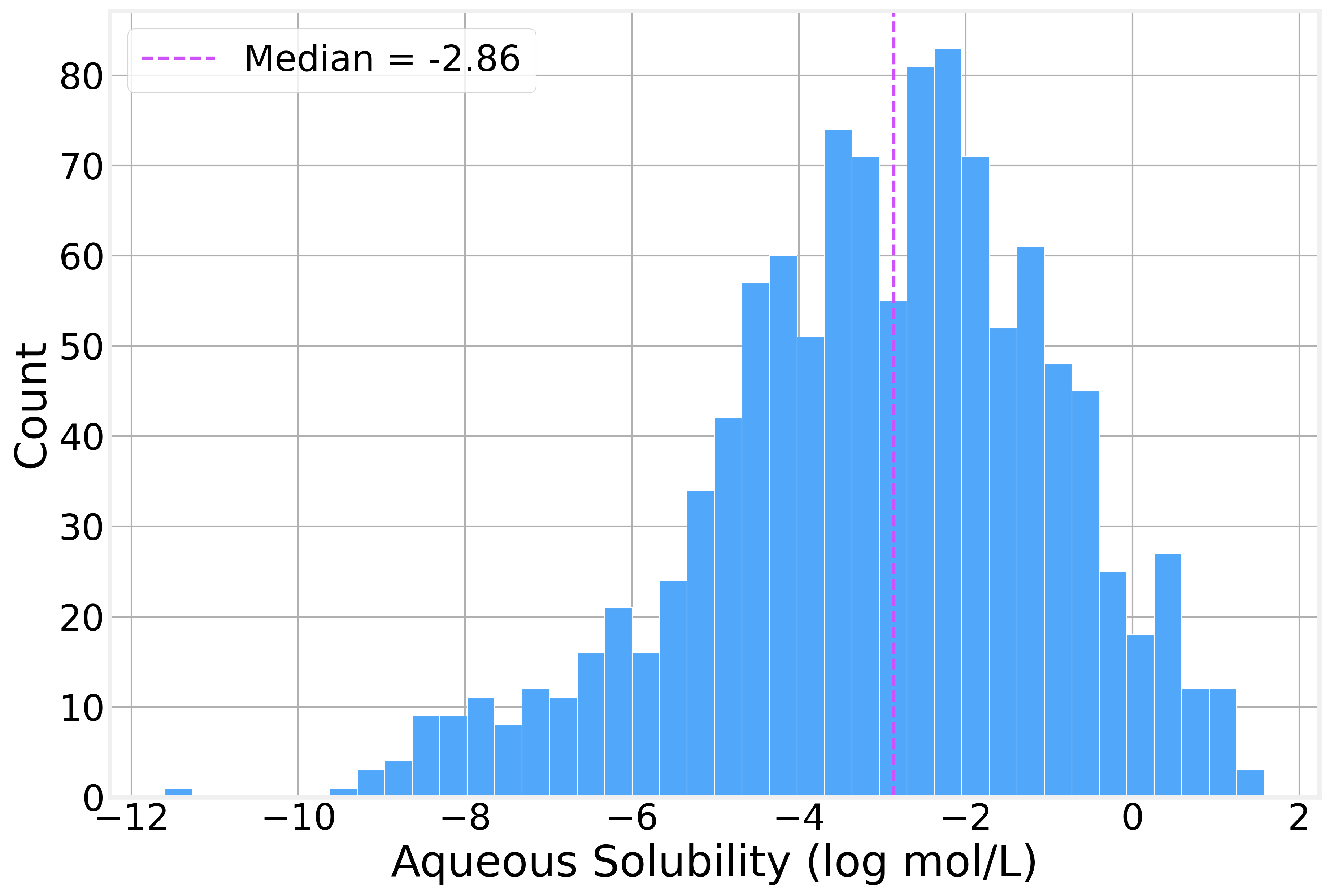
The solubility values span roughly 13 log units, from highly insoluble compounds (around −11.6 log mol/L) to highly soluble ones (+1.58 log mol/L), with a mean of −3.05 and a median of −2.86. The distribution has a rough bell shape with a slight left skew as there are a few *extremely* insoluble molecules pulling the tail.
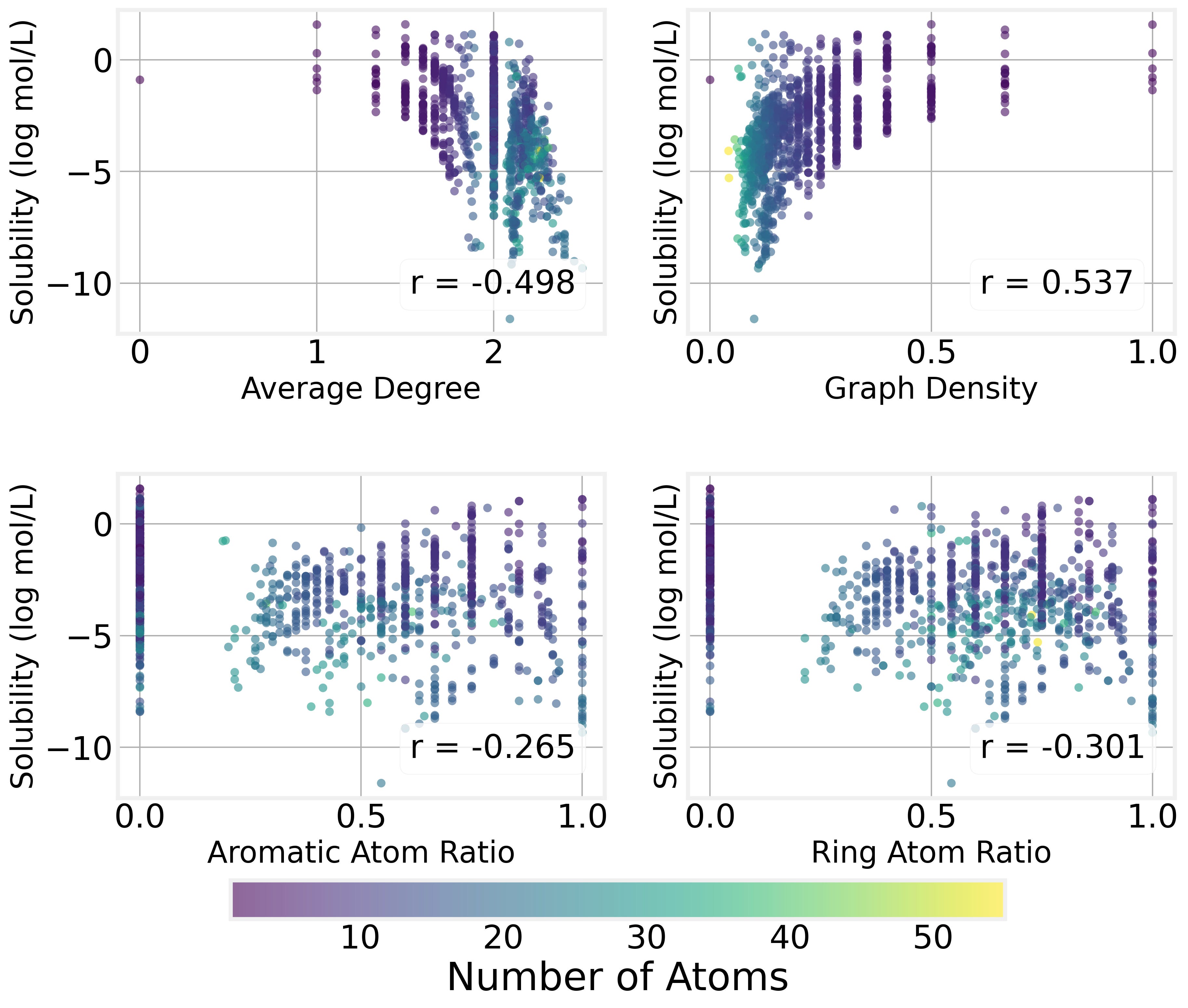
Graph Properties
We can see that the graph structure of the molecule (which atoms are connected) has a strong impact on the solubility by plotting solubility as a function of various connectivity properites:
The Size-Solubility Connection
Perhaps the most intuitive pattern in the data is that bigger molecules tend to be less soluble. The correlation between atom count and solubility is about −0.59. This makes intuitive chemical sense — larger molecules tend to have bigger hydrophobic surfaces that interact poorly with water.
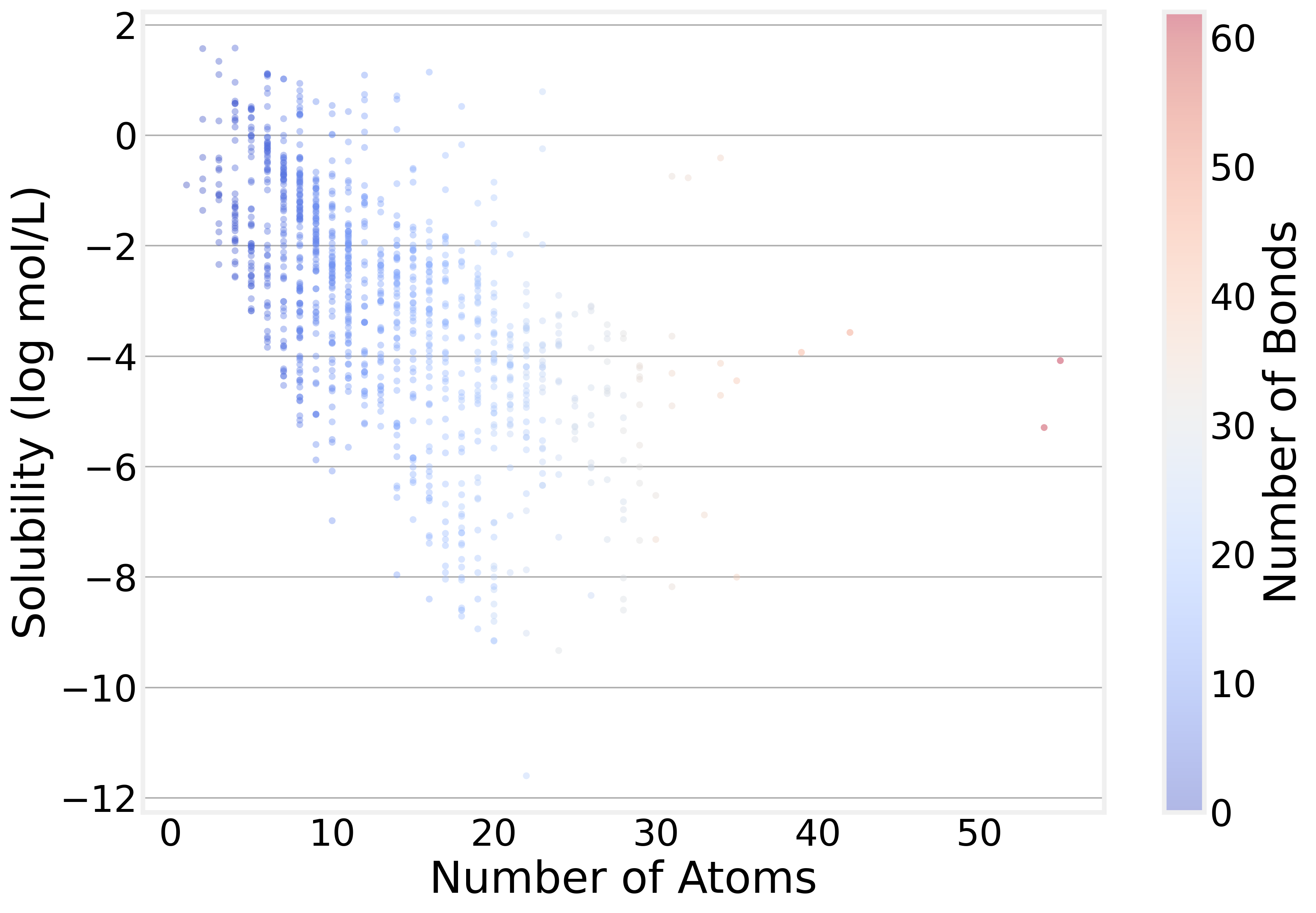
But notice how broad the distribution of solubility is for a specific number of atoms: Molecular size tells part of the story, but nowhere near the whole thing. That’s exactly why we need a model that can look beyond atom counts.
What’s in These Molecules?
Looking at the element distribution across all 14,991 atoms in the dataset, we see exactly what you’d expect from small organic drug-like molecules:
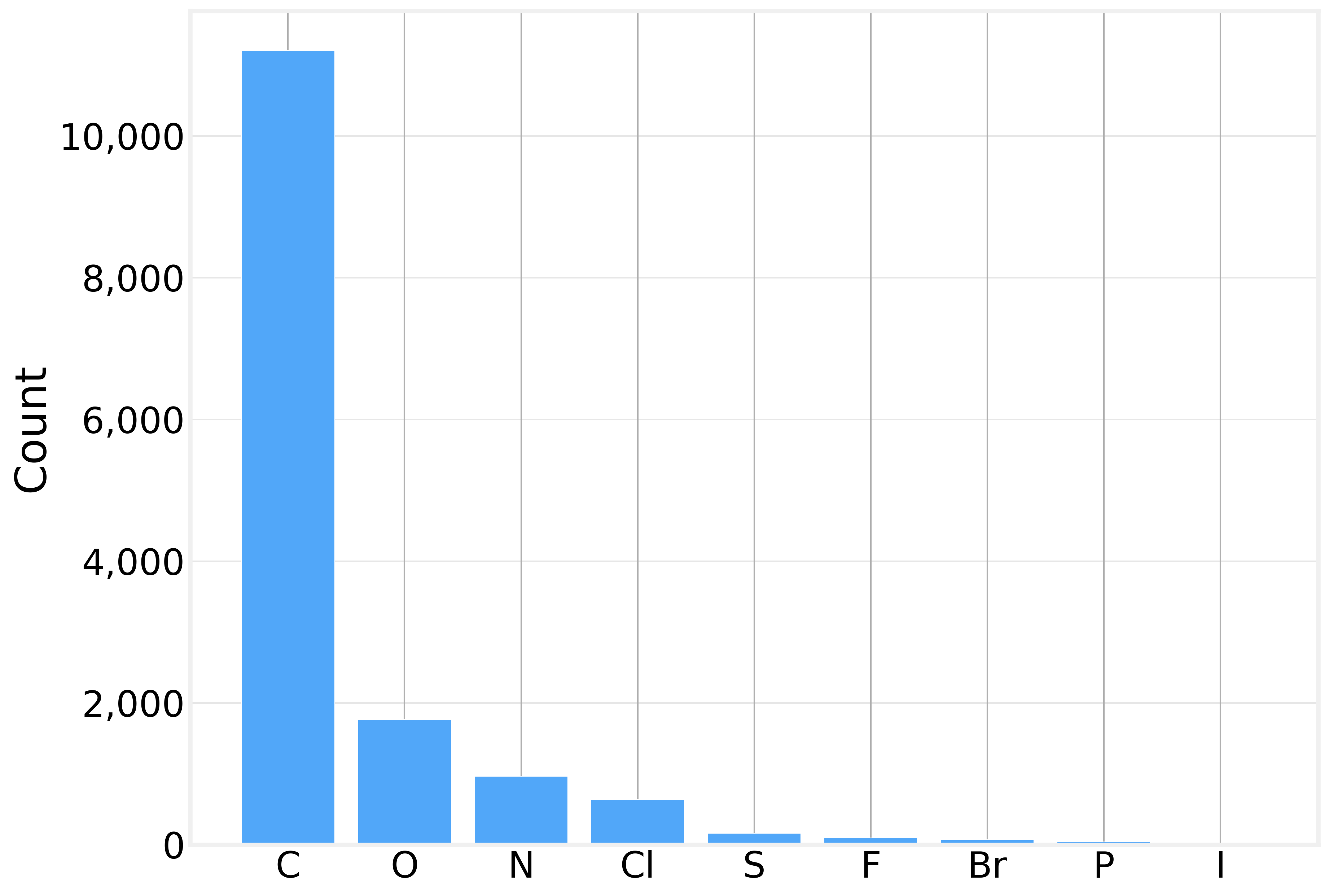
Carbon dominates, as it does in all organic chemistry. The presence of heteroatoms (O, N, S) and halogens (Cl, F, Br, I) is what makes solubility prediction interesting — these atoms introduce polarity, hydrogen bonding potential, and other interactions with water.
Graph Structure
The degree distribution (how many bonds each atom has) peaks sharply at 2, reflecting the prevalence of carbon chains and rings where most atoms have exactly two heavy-atom neighbors. The average degree across all molecules is about 2.06, with a maximum of 4 (think of a fully-substituted carbon).
We can also compute more sophisticated graph metrics for each molecule and examine their correlations with solubility. The strongest predictors turn out to be:
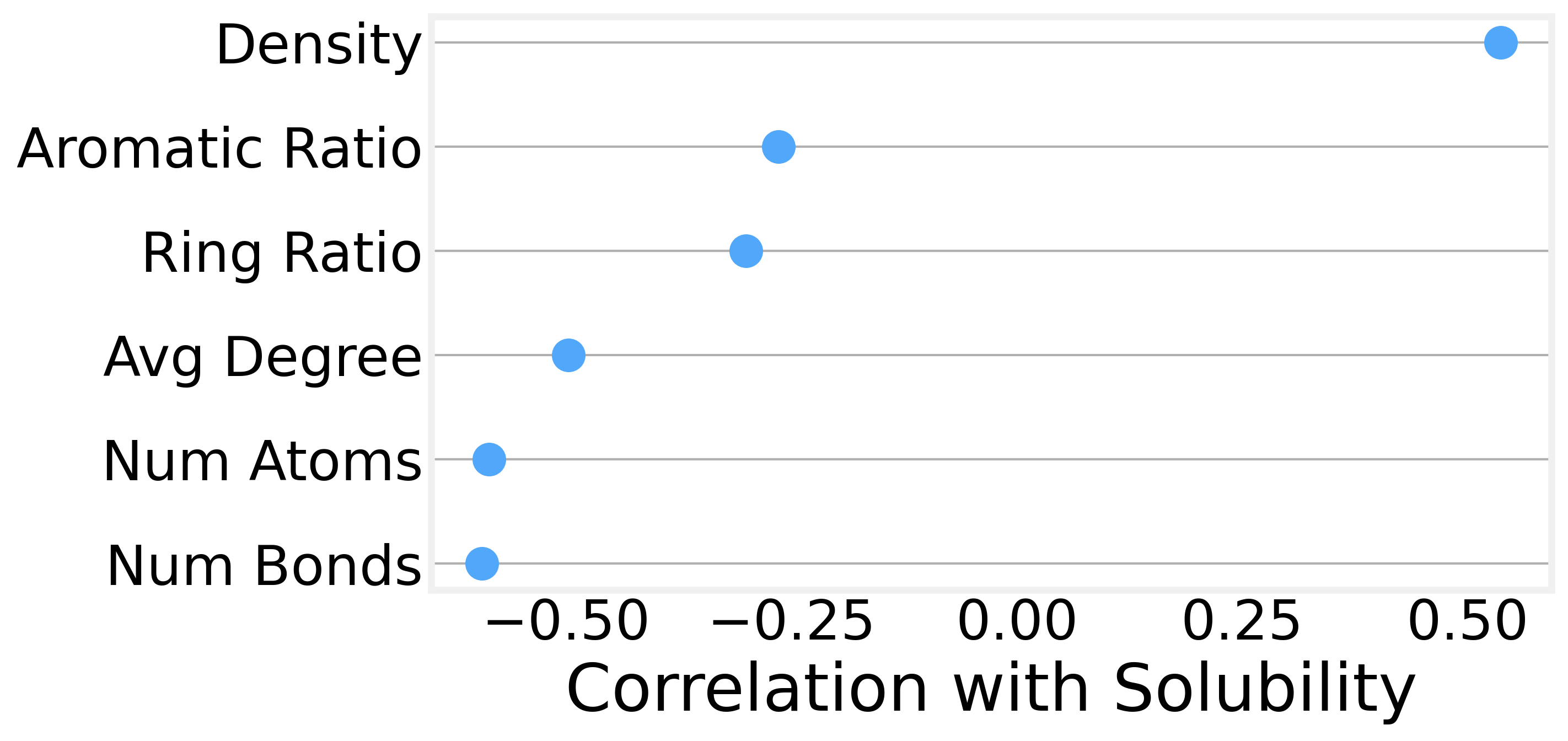
Graph density (the number of edges relative to the maximum possible) is positively correlated with solubility. In other words, size isn’t everything, and denser, more compact molecules tend to be more soluble than sprawling, chain-like ones.
If you’re new to thinking about molecules as graphs, some plots are worth a thousand words. Here is a side-by-side comparison of the same molecule as traditional 2D chemical structures (rendered with RDKit, top) alongside their graph representations (drawn with NetworkX, bottom).
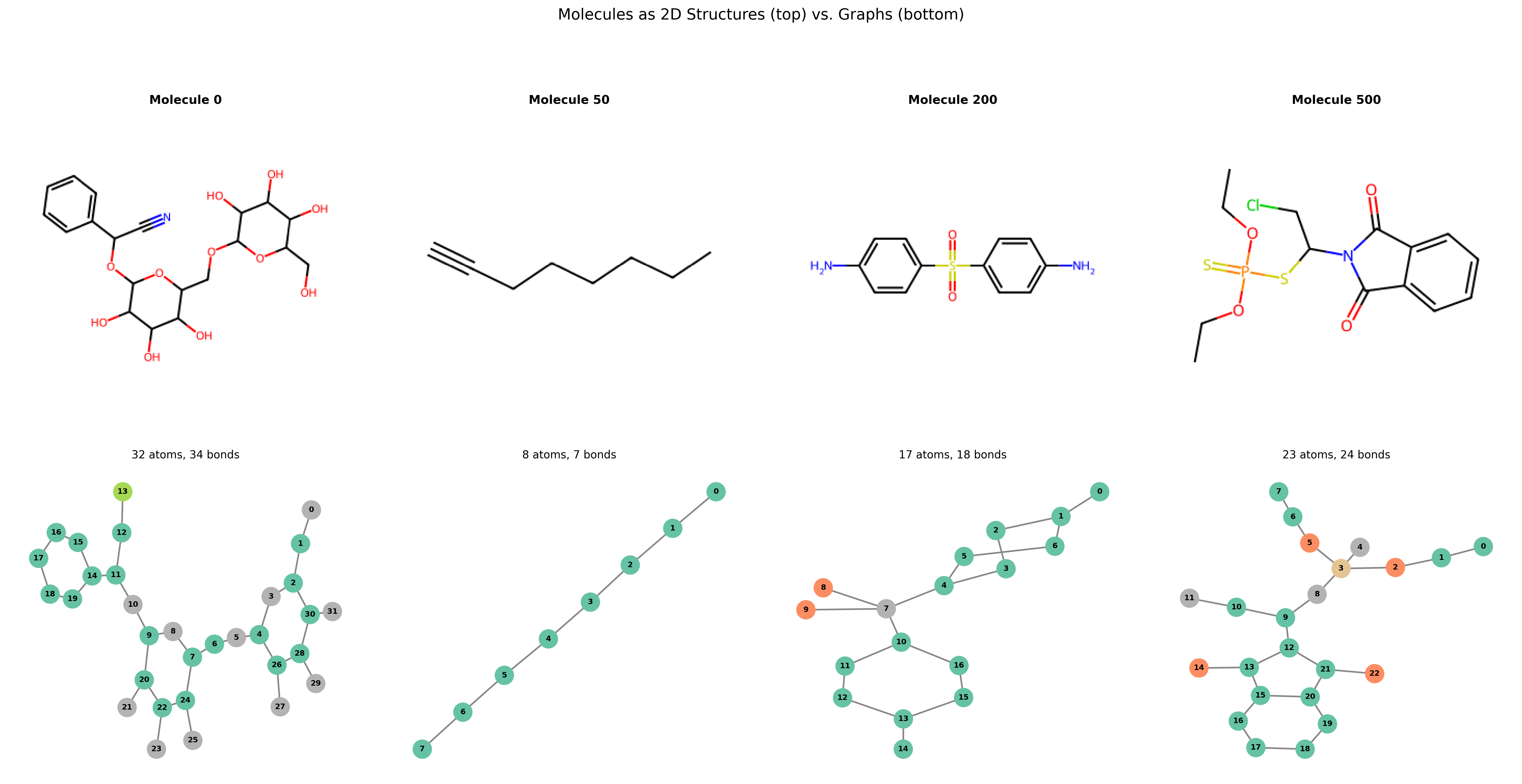
The bottom row looks much friendlier, doesn’t it?
From Atoms to Molecules
A single GCN layer gives each atom information about its immediate neighbors, just one hop away. We stack three layers, one on top of the other, so that each atom’s final representation captures its 3-hop neighborhood. Naturally, the number of layers depends on the typical diameter of your graph, but 3 is more than enough for our purposes.
Now, to move from the properties of a single atom to properties of the whole molecule, we need a way to reduce a variable-length set of atom representations to a single fixed-size vector for the entire graph. This operation is called pooling (also known as graph-level readout).
The simplest and most common choice is to average all the atom feature vectors, a method known as global mean pooling, which has the advantage of not depending on atom ordering, being independent of molecule size, and it works surprisingly well in practice.
After pooling, we feed the resulting vector through a small MLP (multi-layer perceptron) to produce the final solubility prediction:
class MoleculeGNN(nn.Module):
    def __init__(self, num_features, hidden_dim=64, dropout=0.2):
        super().__init__()
        self.conv1 = GCNConv(num_features, hidden_dim)
        self.conv2 = GCNConv(hidden_dim, hidden_dim)
        self.conv3 = GCNConv(hidden_dim, hidden_dim)
        self.mlp = nn.Sequential(
            nn.Linear(hidden_dim, hidden_dim // 2),
            nn.ReLU(),
            nn.Dropout(dropout),
            nn.Linear(hidden_dim // 2, 1)
        )
        self.dropout = dropout

    def forward(self, x, edge_index, batch):
        x = F.relu(self.conv1(x, edge_index))
        x = F.dropout(x, p=self.dropout, training=self.training)
        x = F.relu(self.conv2(x, edge_index))
        x = F.dropout(x, p=self.dropout, training=self.training)
        x = F.relu(self.conv3(x, edge_index))
        x = global_mean_pool(x, batch)   # graph-level readout

        return self.mlp(x).squeeze(-1)
Here it’s worth highlighting the Dropout between GCN layers. Dropout randomly zeros out a fraction of the hidden features during training, preventing co-adaptation and improving generalization, and with just ~900 training molecules, we need all the help we can get.
The entire network has only 11,000 parameters, tiny by modern deep learning standards but convenient for demo purposes and to avoid overfitting to our relatively small dataset.
The full architecture, printed out:
MoleculeGNN(
  (conv1): GCNConv(9, 64)
  (conv2): GCNConv(64, 64)
  (conv3): GCNConv(64, 64)
  (mlp): Sequential(
    (0): Linear(in_features=64, out_features=32, bias=True)
    (1): ReLU()
    (2): Dropout(p=0.2, inplace=False)
    (3): Linear(in_features=32, out_features=1, bias=True)
  )
)
Check out the notebook for a more detailed, but perhaps less illuminating, visualization.
Training the Model
With the architecture in place, training is pretty standard PyTorch fare. We start by splitting the 1,128 molecules 80/10/10 into train (902), validation (113), and test (113) sets using a random permutation.
We train with Adam using MSE loss and early stopping with a patience of 30 epochs to prevent overfitting.
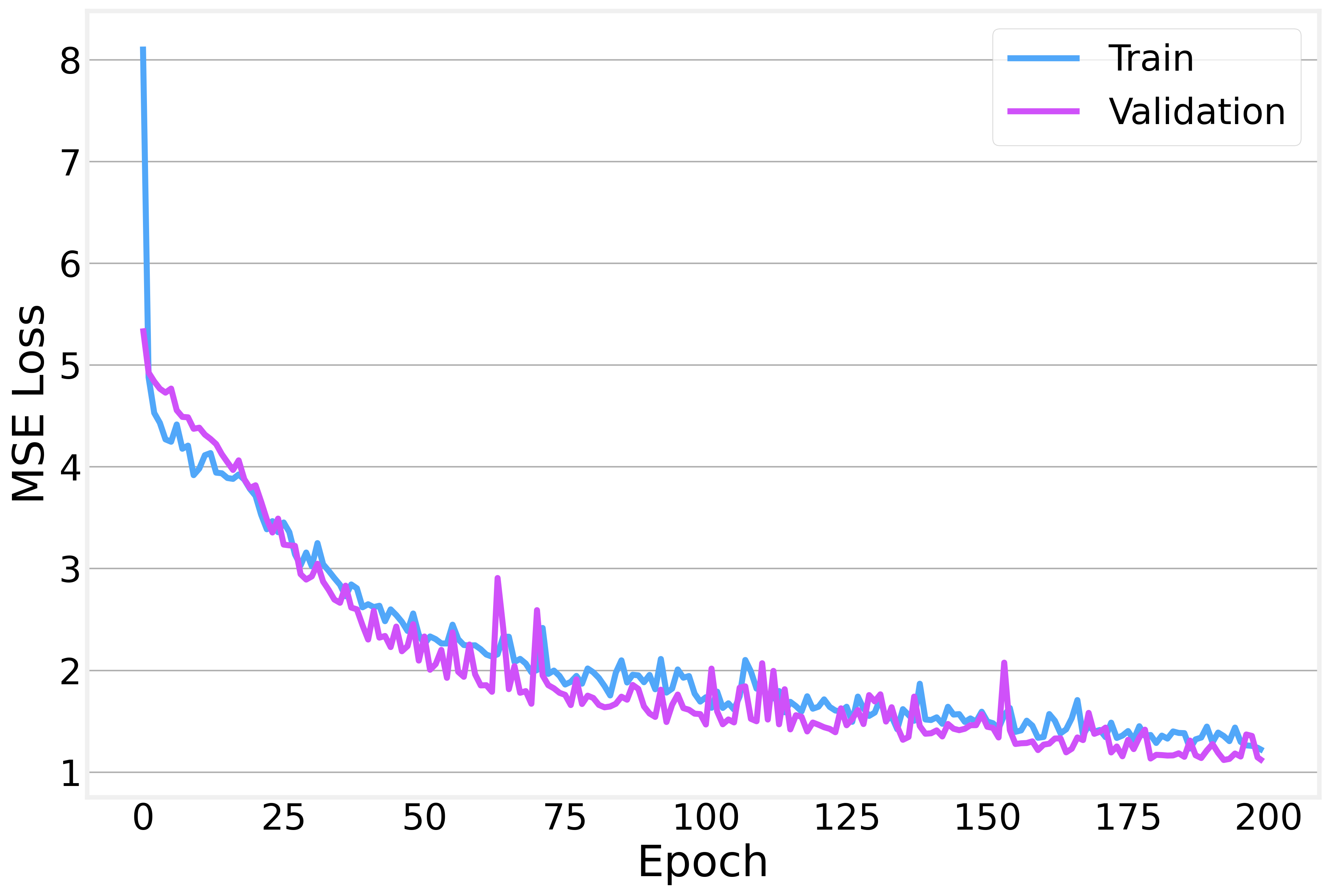
The training and validation losses decrease together nicely, with the gap between them staying relatively small: a sign that we’re not overfitting too badly.
On the held-out test set (113 molecules the model has never seen):
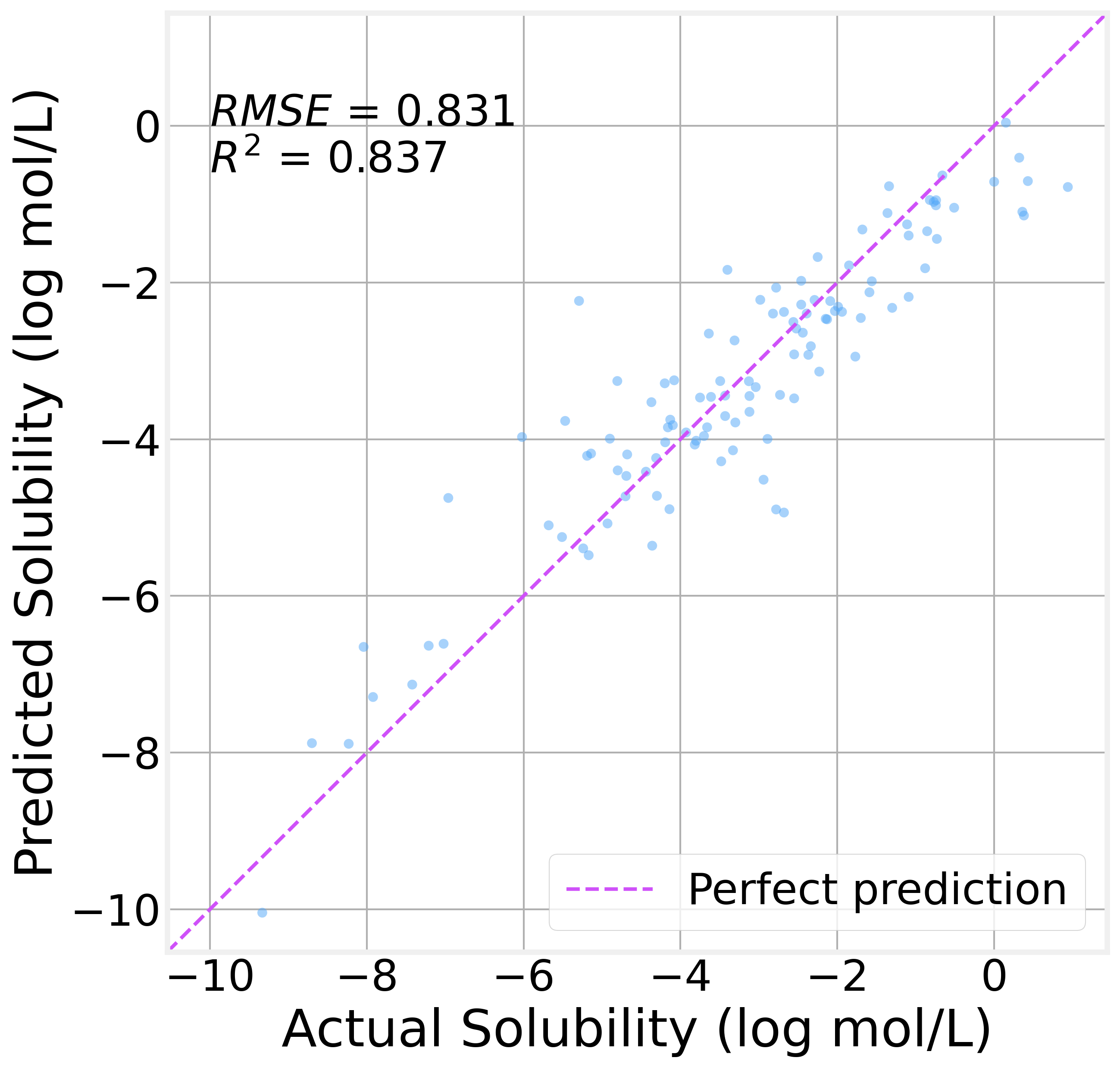
The R² value of 0.84 indicates that the model explains 84% of the variance in solubility. That’s genuinely useful for a model with 11K parameters trained on fewer than a thousand molecules.
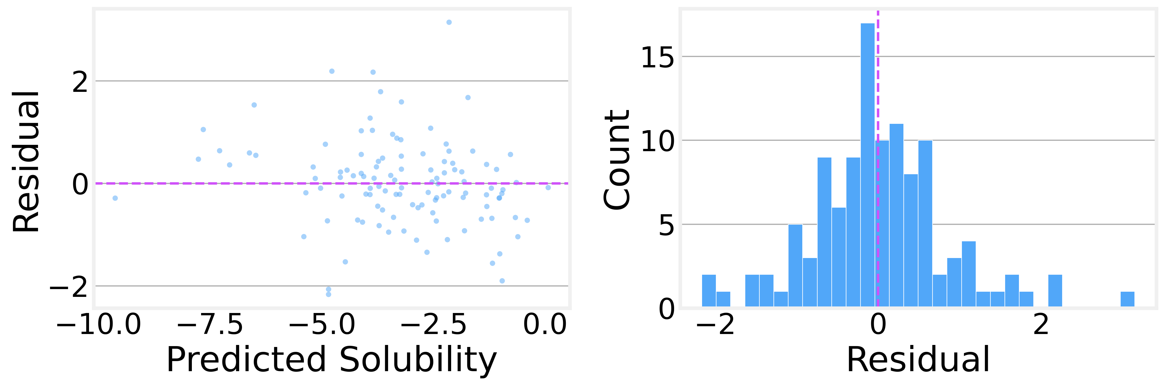
The residual analysis is encouraging, too. The residual distribution is roughly symmetric and centered near zero, with no obvious systematic bias. The residuals-vs-predicted plot shows no strong patterns, suggesting the model isn’t consistently over- or under-predicting in any particular range.
These numbers, while consistent with published GCN baselines on ESOL, are definitely not state-of-the-art. To achieve better results, we would need to use more advanced architectures such as AttentiveFP or SchNet. We kept it simple to avoid obscuring what we’re trying to learn here.
What Did the GNN Learn?
One of the most satisfying things about GNNs is that the intermediate representations, the atom embeddings produced by the GCN layers, are interpretable, at least qualitatively.
After training, we extract the 64-dimensional embedding that the GCN assigns to each atom across our test molecules, then project these 1,385 embeddings down to 2D using t-Distributed Stochastic Neighbor Embedding (t-SNE).

The model has learned to produce chemically meaningful representations without being told any chemistry beyond the raw atomic features (atomic number, degree, etc.). The graph structure encoded by message passing is enough for the model to discover the chemical patterns that matter for solubility on its own. That’s the power of the message passing framework at work.
Beyond Molecules
We used molecules today because they’re a neat example, but everything we built generalizes to any other graph structure. GNNs tackle three broad categories of tasks:
Node-level tasks: Predict something about each node. Classify users in a social network, predict functions of proteins in an interaction graph, and detect anomalous transactions in a financial network.
Edge-level tasks: Predict whether an edge should exist (or what its properties are). Link prediction in social networks, drug-drug interaction prediction, and knowledge graph completion.
Graph-level tasks: Predict a property of the entire graph. Classify molecules, score protein structures, and assess network robustness.
For graph-level tasks (like the one we explored today), the key ingredient is the readout operation. We used global mean pooling (averaging all node embeddings), but there are other options: sum pooling (preserves information about the graph size), max pooling (captures the most active features), or even learned hierarchical pooling that progressively coarsens the graph.
We hope you enjoyed this Graphs post on the Data for Science Substack and look forward to hearing your thoughts. We hope you
You can find all the code for the analysis in this post in our companion GitHub Repository https://github.com/DataForScience/Graphs4Sci
And, of course, don’t forget to
this post with others who might be interested, and encourage them to
so that they have access to the entire backlog of posts and be the first to know when a new a new article is posted.